Optical pooled screens

An optical pooled screen (OPS) delivers a CRISPR library to one dish of cells, images every cell in a few channels, and reads each cell’s guide by in-situ sequencing. One dish holds thousands of knockouts at once. The payoff is a map: because genes that do the same job in the cell look alike under the microscope, morphology alone rediscovers the cell’s machinery, the ribosome, the proteasome and the spliceosome among it, with no sequence or annotation used.

This page builds to that map on Aconcagua, a reanalysis of a HeLa CRISPR screen of 5,072 fitness-conferring genes (Funk et al. 2022) imaged in four channels: DNA (DAPI), microtubules (alpha-tubulin), DNA damage (gamma-H2AX) and F-actin (phalloidin). It first works a subset end to end, from a single cell to a gene call, with mantispy, meeting the one problem an OPS has to get right along the way: the DNA damage that Cas9 causes simply by cutting. It then opens the full published landscape and shows what morphology recovers.

Two words recur. A guide is one CRISPR reagent against one gene; four guides target each gene, and a guide is the unit that is scored. A well is one imaged culture; because the library is pooled, every well holds many guides, and a guide’s wells are its replicates. The data come from the Brieflow reanalysis by Di Bernardo et al., Nat Commun 17, 6997 (2026), doi:10.1038/s41467-026-73643-7, of the screen in Funk et al., Cell 185, 4634 (2022), and served through the CZ Biohub OPS Explorer.

import warnings

import anndata as ad
import matplotlib.pyplot as plt
import numpy as np
import pandas as pd
import pooch
import scanpy as sc

import mantispy as mt

warnings.filterwarnings("ignore")
sc.settings.verbosity = 0
plt.rcParams["figure.dpi"] = 110
SEED = 0

adata = mt.ds.aconcagua()
adata

AnnData object with n_obs × n_vars = 84125 × 1483
    obs: 'Metadata_Plate', 'Metadata_Well', 'Metadata_sgRNA', 'Metadata_CellCount', 'Metadata_SiteCount', 'Metadata_Gene', 'Metadata_Perturbation', 'Metadata_Perturbation_Type', 'Metadata_Control_Type', 'Metadata_Tier', 'Metadata_Control', 'Metadata_Row', 'Metadata_Col', 'Metadata_ObjectType', 'Metadata_MitoticFraction'
    var: 'object', 'feature_group', 'feature', 'channel', 'scale', 'angle', 'gray_levels', 'radial_bin', 'params', 'is_feature', 'feature_kind', 'degenerate_scale'
    uns: 'mantispy'
    layers: None (.X)

One row per guide per well: the median of that guide’s cells in that well, normalized against the non-targeting cells of the same well with normalize(). The subset keeps all 250 non-targeting guides, four positive controls, 50 strong and 50 weak known hits, and 396 random library genes, each as profiles across 46 wells.

Figures and image helpers

The functions below draw every figure on this page and fetch the example cell crops from the OPS Explorer bucket. They hold no analysis, only plotting and downloading, so the cells that follow stay a short prep, the mantispy call, and a plot. Skip to the next section for the first step. Fetching crops needs boto3 and zarr, which the core package does not require.

import boto3
import zarr
from botocore import UNSIGNED
from botocore.config import Config

CHANNELS = ["DNA (DAPI)", "microtubules", "gamma-H2AX", "F-actin"]
_S3 = boto3.client("s3", region_name="us-west-2", config=Config(signature_version=UNSIGNED))
_BUCKET = "ops-explorer-public"
_CROPS = pooch.os_cache("mantispy") / "aconcagua_crops"


def _prefixes(prefix):
    out, token = [], None
    while True:
        extra = {"ContinuationToken": token} if token else {}
        r = _S3.list_objects_v2(Bucket=_BUCKET, Prefix=prefix.rstrip("/") + "/", Delimiter="/", **extra)
        out += [p["Prefix"] for p in r.get("CommonPrefixes", [])]
        if not r.get("IsTruncated"):
            return out
        token = r["NextContinuationToken"]


def example_cells(gene, n=4, phase="interphase", seed=SEED):
    """Return n (4, H, W) crops for a gene, downloaded once and cached locally."""
    base = f"aconcagua/aconcagua/visualizations/{phase}/examples/DAPI_TUBULIN_GH2AX_PHALLOIDIN"
    guide = _prefixes(f"{base}/{gene}")[0].rstrip("/")
    crops = _prefixes(guide)
    picks = np.random.default_rng(seed).choice(len(crops), size=min(n, len(crops)), replace=False)
    images = []
    for i in sorted(picks):
        crop = crops[i].rstrip("/")
        local = _CROPS / crop
        if not (local / "zarr.json").exists():
            local.mkdir(parents=True, exist_ok=True)
            for obj in _S3.list_objects_v2(Bucket=_BUCKET, Prefix=crop + "/")["Contents"]:
                dst = _CROPS / obj["Key"]
                dst.parent.mkdir(parents=True, exist_ok=True)
                _S3.download_file(_BUCKET, obj["Key"], str(dst))
        images.append(np.asarray(zarr.open_group(str(local), mode="r")["0"][:]).squeeze())
    return images


def _stretch(plane):
    lo, hi = np.percentile(plane, [1, 99.5])
    return np.clip((plane.astype(float) - lo) / max(hi - lo, 1), 0, 1)


def show_cells(images, title):
    """Draw each cell as a row of its four channels."""
    fig, axes = plt.subplots(len(images), 4, figsize=(8, 2 * len(images)), squeeze=False)
    for row, img in enumerate(images):
        for col in range(4):
            ax = axes[row, col]
            ax.imshow(_stretch(img[col]), cmap="magma")
            ax.set_xticks([])
            ax.set_yticks([])
            if row == 0:
                ax.set_title(CHANNELS[col], fontsize=9)
    fig.suptitle(title)
    fig.tight_layout()
    plt.show()


def plot_controls(adata):
    """Boxplots: each positive control against the non-targeting cells, in its own channel."""
    controls = (adata.obs["Metadata_Control_Type"] == "negcon").to_numpy()
    checks = {
        "H2AX": ("Nuclei_Intensity_MeanIntensity_GH2AX", "gamma-H2AX"),
        "TUBB": ("Cells_Intensity_MeanIntensity_TUBULIN", "tubulin"),
        "CFL1": ("Cells_Intensity_MeanIntensity_PHALLOIDIN", "F-actin"),
    }
    fig, axes = plt.subplots(1, 3, figsize=(9, 3.2), sharey=True)
    for ax, (gene, (feature, label)) in zip(axes, checks.items(), strict=True):
        values = adata[:, feature].X.ravel()
        ko = values[(adata.obs["Metadata_Gene"] == gene).to_numpy()]
        ntc = values[controls]
        ax.boxplot([ntc, ko], tick_labels=["NTC", f"{gene} KO"], widths=0.6, showfliers=False)
        ax.axhline(0, color="0.7", lw=0.8, zorder=0)
        ax.set_title(f"{gene}\n({label})", fontsize=9)
    axes[0].set_ylabel("robust z (guide x well)")
    fig.suptitle("Positive controls shift the channel they were chosen for")
    fig.tight_layout()
    plt.show()


def plot_damage(damage):
    """Boxplots of brightest gamma-H2AX focus by gene kind, non-targeting through positive control."""
    groups = ["non-targeting", "unexpressed", "random", "weak", "strong", "positive_control"]
    fig, ax = plt.subplots(figsize=(6.5, 3.6))
    ax.boxplot([damage.loc[damage["kind"] == g, "z"] for g in groups], tick_labels=groups, showfliers=False, widths=0.6)
    ax.axhline(0, color="0.7", lw=0.8, zorder=0)
    ax.set_ylabel("brightest gamma-H2AX focus (z)")
    ax.set_title("Even unexpressed genes carry more DNA damage than not cutting")
    plt.setp(ax.get_xticklabels(), rotation=20, ha="right")
    fig.tight_layout()
    plt.show()


def plot_rates(rates):
    """Grouped bars: fraction of each tier called, against non-targeting and beyond cutting."""
    ax = rates.plot.bar(figsize=(6.5, 3.8), color=["#9ecae1", "#e6550d"], rot=0)
    ax.set_ylabel("fraction called")
    ax.set_ylim(0, 1)
    ax.set_title("Against the cut, the random-gene rate collapses while the strong hits stay")
    ax.legend()
    plt.show()


def plot_phase(phase):
    """Stacked bars of cell-cycle phase per knockout."""
    fig, ax = plt.subplots(figsize=(6.5, 3.8))
    bottom = np.zeros(len(phase))
    colours = {"sub-2N": "#bdbdbd", "G1": "#9ecae1", "S": "#fdae6b", "G2M": "#e6550d", "above-4N": "#756bb1"}
    for col, color in colours.items():
        if col not in phase:
            continue
        ax.bar(phase.index, phase[col], bottom=bottom, color=color, label=col)
        bottom += phase[col].to_numpy()
    ax.set_ylabel("fraction of cells")
    ax.set_title("Cell-cycle phase by knockout")
    ax.legend(title="phase", bbox_to_anchor=(1.01, 1), loc="upper left")
    plt.setp(ax.get_xticklabels(), rotation=30, ha="right")
    fig.tight_layout()
    plt.show()


def plot_complex_blocks(S, pos, members, bounds, labels, random_pairs):
    """Left: correlation block of top complexes. Right: subunit correlation vs the random baseline."""
    block = S[np.ix_([pos[g] for g in members], [pos[g] for g in members])]
    fig, axes = plt.subplots(1, 2, figsize=(11, 5), gridspec_kw={"width_ratios": [1.15, 1]})
    im = axes[0].imshow(block, cmap="RdBu_r", vmin=-1, vmax=1)
    for b in bounds[1:-1]:
        axes[0].axhline(b - 0.5, color="k", lw=0.6)
        axes[0].axvline(b - 0.5, color="k", lw=0.6)
    ticks = [(bounds[i] + bounds[i + 1]) / 2 - 0.5 for i in range(len(labels))]
    axes[0].set_xticks(ticks, labels, rotation=30, ha="right", fontsize=7)
    axes[0].set_yticks(ticks, labels, fontsize=7)
    fig.colorbar(im, ax=axes[0], shrink=0.7, label="profile correlation")
    axes[0].set_title("Complex subunits correlate within, not across")

    families = {"ribosome": ("RPL", "RPS"), "proteasome": ("PSM",), "spliceosome": ("SNRP", "SF3")}
    data, names = [random_pairs], ["random"]
    for name, pref in families.items():
        m = [pos[g] for g in pos if str(g).startswith(pref)]
        sub_s = S[np.ix_(m, m)]
        data.append(sub_s[np.triu_indices(len(m), 1)])
        names.append(f"{name}\n(n={len(m)})")
    axes[1].boxplot(data, tick_labels=names, showfliers=False, widths=0.6)
    axes[1].axhline(float(np.mean(random_pairs)), color="0.6", ls=":", lw=1)
    axes[1].set_ylabel("profile correlation")
    axes[1].set_title("Subunits vs the random baseline")
    fig.tight_layout()
    plt.show()


def plot_cluster_names(modules):
    """Horizontal bars of the strongest cluster-to-complex enrichments."""
    tab = modules.tail(12)
    fig, ax = plt.subplots(figsize=(7.5, 4.5))
    ax.barh(range(len(tab)), tab["neglog10q"], color="#31a354")
    ax.set_yticks(
        range(len(tab)),
        [f"{c[:34]}  ({k}/{s})" for c, k, s in zip(tab["complex"], tab["k"], tab["size"], strict=True)],
        fontsize=8,
    )
    ax.set_xlabel("enrichment -log10 q")
    ax.set_title("Morphological clusters map to CORUM complexes")
    fig.tight_layout()
    plt.show()


def plot_candidates(picks, S, pos, random_pairs):
    """Per complex: each candidate gene's correlation to known members, against the member and random levels."""
    fig, axes = plt.subplots(1, len(picks), figsize=(4 * len(picks), 4), sharey=True)
    for ax, (cx, known, cand) in zip(np.atleast_1d(axes), picks, strict=True):
        ki = [pos[g] for g in known]
        base = float(np.mean(random_pairs))
        member_level = float(np.mean([S[np.ix_(ki, ki)][np.triu_indices(len(ki), 1)]]))
        vals = [float(np.mean([S[pos[g], j] for j in ki])) for g in cand]
        ax.axhline(member_level, color="#31a354", ls="-", lw=1.5, label="complex members")
        ax.axhline(base, color="0.6", ls=":", lw=1, label="random")
        ax.bar(range(len(cand)), vals, color="#e6550d")
        ax.set_xticks(range(len(cand)), cand, rotation=40, ha="right", fontsize=8)
        ax.set_title(cx[:28], fontsize=9)
    axes[0].set_ylabel("correlation to known members")
    axes[0].legend(fontsize=7, loc="lower right")
    fig.suptitle("Candidate partners placed into their complex by morphology")
    fig.tight_layout()
    plt.show()


def plot_machines(corum_coherent, hallmark_coherent, recall, null):
    """Left: fraction coherent, CORUM vs hallmark. Right: CORUM co-member recall against the permutation null."""
    fig, axes = plt.subplots(1, 2, figsize=(8.5, 3.8))
    axes[0].bar(
        ["CORUM\ncomplexes", "hallmark\nprograms"],
        [corum_coherent, hallmark_coherent],
        color=["#e6550d", "#9ecae1"],
    )
    axes[0].set_ylabel("fraction coherent (q < 0.05)")
    axes[0].set_ylim(0, 1)
    axes[0].set_title("Morphology recovers machines, not programs")
    axes[1].bar(["observed", "chance"], [recall, null], color=["#e6550d", "0.6"])
    axes[1].set_ylabel("CORUM co-member pairs in the tails")
    axes[1].set_title("Complex co-members recalled above chance")
    fig.tight_layout()
    plt.show()

What the screen sees

Before any profile, the cells. The OPS Explorer publishes example crops of segmented cells, one small OME-Zarr per cell in four channels. A handful for one gene shows what every feature below is measured from: the nucleus in DNA, the spindle in tubulin, double-strand breaks in gamma-H2AX, the cell body in actin.

show_cells(example_cells("CFL1"), "Four channels of one guide's cells (CFL1)")

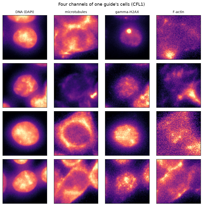
Each row is one cell; each column a channel. Every feature that follows is a summary of images like these.

The controls move the channel they were chosen for

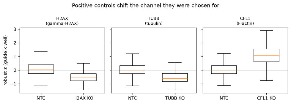
Before calling anything, a sanity check: the screen’s own positive controls should move the channel they were chosen for. The knockouts of H2AX, TUBB and CFL1 remove or disturb the very protein a stain detects, so each should shift its feature away from the non-targeting cells. They do, in the expected direction.

plot_controls(adata)

The calling that follows is kept honest in ways we will not dwell on: degenerate features with no spread are dropped (feature_select()), the subset was drawn so controls and targeting guides carry comparable cell counts, and each well is normalized against its own non-targeting cells, which leaves no plate or well effect for a batch correction to remove. With that in place, the one problem specific to a CRISPR screen is next.

Cas9 cutting is a phenotype of its own

A targeting guide makes Cas9 cut the genome; a non-targeting guide does not. The double-strand break alone raises gamma-H2AX, whatever gene is cut, so a guide can look active just for cutting. Genes the cells do not express are the clean test: knocking them out can do nothing, yet they still carry more DNA damage than not cutting at all. DepMap’s expression for HeLa (model ACH-001086) names the unexpressed genes.

mt.pp.feature_select(adata)
adata = mt.pp.subset_features(adata)

WARNING  feature_select: 12 selected feature(s) lie more than 500 robust standard deviations from their median     
         (Cells_Intensity_WeightedHuMoment5_DAPI, Cells_Intensity_WeightedHuMoment5_TUBULIN,                       
         Cells_AreaShape_HuMoment_4, Cells_AreaShape_HuMoment_5, Cells_AreaShape_HuMoment_6 and 7 more)            

unexpressed = mt.io.unexpressed_genes(mt.ds.depmap_expression(), "ACH-001086")

foci = "Nuclei_Intensity_MaxIntensity_GH2AX"
go = adata.obs
kind = np.where(
    go["Metadata_Control_Type"] == "negcon",
    "non-targeting",
    np.where(go["Metadata_Gene"].astype(str).isin(unexpressed), "unexpressed", go["Metadata_Tier"].astype(str)),
)
damage = pd.DataFrame({"z": adata[:, foci].X.ravel(), "kind": kind})
plot_damage(damage)

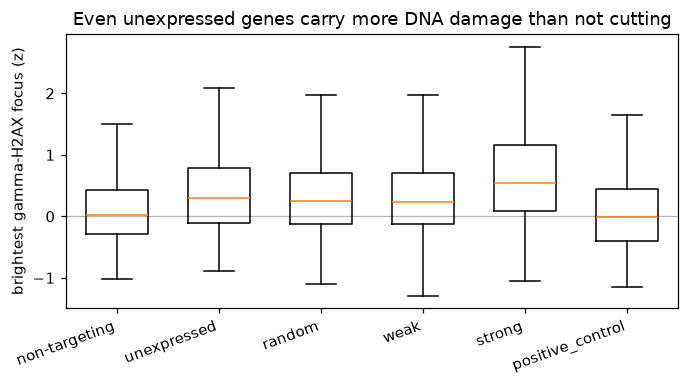
So a non-targeting null answers does this guide differ from not cutting. The question a screen asks is does losing this gene do anything beyond the cut, and the unexpressed genes are its null. Pooling each gene’s four guides into a call (guide_activity(), aggregate_guides()) and then calibrating against the unexpressed genes (empirical_fdr()) separates the two. The non-targeting guides are split at random so the activity scale is set on one half and the null on the other, never on themselves.

The feature_select() warning above names twelve Hu-moment features with extreme values in a few guide-by-well profiles. They are kept, because in the per-guide medians the calls are made from they stay within the range of the other features, as the first line below shows.

guides = mt.tl.aggregate(adata, by=("Metadata_sgRNA",), func="median", min_cells=1)
go = guides.obs
ntc = np.sort(go.loc[go["Metadata_Control_Type"] == "negcon", "Metadata_sgRNA"].astype(str).unique())
roll = np.random.default_rng(SEED).permutation(ntc)
role = dict.fromkeys(roll[:100], "ntc_scale") | dict.fromkeys(roll[100:200], "nontargeting")
role |= {guide: f"PSEUDO{i // 4:02d}" for i, guide in enumerate(roll[200:248])}
assigned = go["Metadata_sgRNA"].astype(str).map(role)
go["Analysis_Group"] = np.where(assigned.notna(), assigned, go["Metadata_Gene"].astype(str))
guides.X = np.nan_to_num(guides.X)
hu = guides.var_names.str.contains("HuMoment")
print(
    f"largest |value| over guides: Hu moments {np.abs(guides.X[:, hu]).max():.1f}, other features {np.abs(guides.X[:, ~hu]).max():.1f}"
)
sc.pp.pca(guides, n_comps=50, random_state=SEED)

largest |value| over guides: Hu moments 7.3, other features 20.4

mt.tl.guide_activity(guides, reference="ntc_scale", group="Analysis_Group", use_rep="X_pca")
mt.tl.aggregate_guides(
    guides, score="guide_activity", guide="Metadata_sgRNA", gene="Analysis_Group", control="nontargeting", seed=SEED
)
calls = pd.DataFrame(guides.uns["mantispy"]["gene_aggregation"]).set_index("group").rename_axis("gene")
tier = dict(zip(go["Metadata_Gene"].astype(str), go["Metadata_Tier"].astype(str), strict=True))
calls["tier"] = ["pseudo-gene" if g.startswith("PSEUDO") else tier.get(g, "?") for g in calls.index]
calls["unexpressed"] = calls.index.isin(unexpressed)

genes = calls[calls["tier"] != "pseudo-gene"].copy()
table = ad.AnnData(obs=pd.DataFrame({"gene": genes.index, "score": genes["statistic"].to_numpy()}, index=genes.index))
mt.tl.empirical_fdr(
    table, control_genes=sorted(set(genes.index) & unexpressed), score="score", group="gene", alpha=0.05, criterion="q"
)
beyond = pd.DataFrame(table.uns["mantispy"]["empirical_fdr"]).set_index("group")
genes["beyond_cutting"] = beyond["is_hit"].reindex(genes.index).astype("boolean")

WARNING  empirical_fdr: only 32 control genes are present, so the false discovery rate can take only a few values  

tested = genes[~genes["unexpressed"]]
rates = tested.groupby("tier").agg(
    **{"vs non-targeting": ("is_hit", "mean"), "beyond cutting": ("beyond_cutting", "mean")}
)
rates = rates.reindex(["positive_control", "strong", "weak", "random"]).dropna(how="all")
count = tested["tier"].value_counts()
rates.index = [f"{tier}\n(n={count[tier]})" for tier in rates.index]
pseudo = calls[calls["tier"] == "pseudo-gene"]
print(f"pseudo-genes called against non-targeting: {int(pseudo['is_hit'].sum())} of {len(pseudo)}")
plot_rates(rates)

pseudo-genes called against non-targeting: 0 of 12

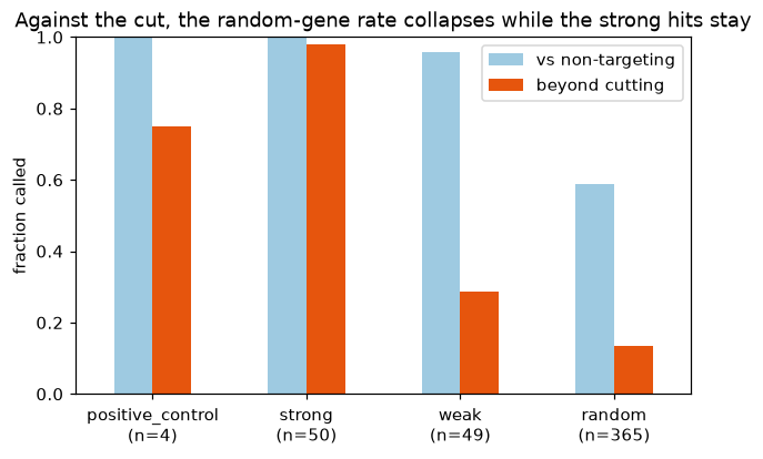
Against the unexpressed null the strong known hits mostly stay, while the rates of the weak hits and the random genes fall sharply. The strong hits survive because they do something beyond cutting; most weak hits and random genes show nothing beyond it here. Three of the four positive controls stay, too few to read as a rate. None of the twelve pseudo-genes, each four non-targeting guides grouped at random, is called against the non-targeting null, so the calling does not make genes out of control guides. (The unexpressed genes are few, so the null is coarse, which is why the cutoff is a q-value of 0.05 rather than anything finer. Replication of a gene’s guides against a permutation null can be measured a different way, via percent_replicating().)

What moved

A call says a gene does something; the features say what. A moderated t-test per feature against the controls (differential_features()) collapsed by channel (feature_signature()) gives a compact fingerprint per gene.

examples = ["RRM1", "DTL", "SKA2", "HAUS6", "ITGAV", "TLN1", "PSMB7", "SF3B3"]
present = [g for g in examples if (adata.obs["Metadata_Gene"].astype(str) == g).any()]
negcon = list(adata.obs.loc[adata.obs["Metadata_Control_Type"] == "negcon", "Metadata_Gene"].astype(str).unique())
sub = adata[adata.obs["Metadata_Gene"].astype(str).isin(present + negcon)].copy()
mt.tl.differential_features(sub, groupby="Metadata_Gene", reference="negcon", block="Metadata_Plate")
sig = mt.tl.feature_signature(sub, key="differential", by=("channel",), statistic="t")
sig = sig[[g for g in present if g in sig.obs_names]].copy()

fig, ax = plt.subplots(figsize=(7, 4))
mt.pl.feature_signature(sig, top=sig.n_vars, ax=ax)
ax.set_title("Which channel each knockout moved")
fig.tight_layout()
plt.show()

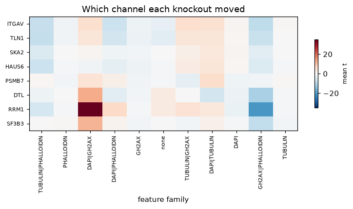
Replication-stress genes (RRM1, DTL) light up gamma-H2AX and DNA, the spindle genes (SKA2, HAUS6) tubulin, and the adhesion genes (ITGAV, TLN1) actin. The proteasome subunit PSMB7 and the spliceosome subunit SF3B3 add two more. The fingerprint is what turns a hit into a hypothesis.

Inside the well: single cells

A profile is a median over a well’s cells, but a knockout rarely moves every cell the same way. The published subset keeps the single cells for eight genes plus controls, with raw intensities. 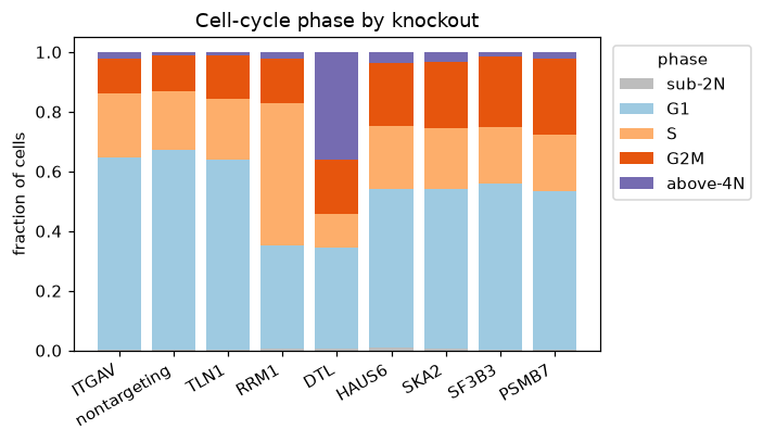Integrated DNA intensity roughly doubles from G1 to G2M, so dna_content() reads each cell’s DNA against the G1 peak of the non-targeting cells in its well, and fit_cell_cycle() and project_cell_cycle() call its phase from that, with cells below 2N and above 4N kept apart. The knockouts move cells to different phases, which a well median would blur into a single number: more of RRM1’s cells sit in S than the controls’, more of DTL’s above 4N, and more of the spindle knockouts’ in G2M.

cells = mt.ds.aconcagua_cells()
mt.tl.dna_content(cells, dna_feature="Nuclei_Intensity_IntegratedIntensity_DAPI", reference="negcon")
mt.tl.fit_cell_cycle(cells)
mt.tl.project_cell_cycle(cells)
wells = cells.uns["mantispy"]["cell_cycle_wells"]
print("not judged:", wells.loc[wells["shift"].isna(), ["Metadata_Plate", "Metadata_Well"]].to_numpy().tolist())

phase = pd.crosstab(cells.obs["Metadata_Gene"], cells.obs["cell_cycle_phase"], normalize="index")
phase = phase.sort_values("G2M")
plot_phase(phase)

not judged: [['6', 'B01'], ['7', 'A02']]

# Each well holds every guide, so test the phase shares within each plate's wells and relabel whole guides for the null.
mt.tl.composition_shift(
    cells, key="cell_cycle_phase", groupby="Metadata_Gene", replicate="Metadata_sgRNA", n_permutations=999
)
shift = cells.uns["mantispy"]["composition_shift"].set_index("group")
shift[["G1", "S", "G2M", "above-4N", "distance", "n_blocks", "pvalue", "qvalue", "min_pvalue"]].sort_values(
    "G2M", ascending=False
).round(3)

	G1	S	G2M	above-4N	distance	n_blocks	pvalue	qvalue	min_pvalue
group
PSMB7	-0.137	-0.008	0.136	0.010	0.146	46	0.005	0.010	0.001
SF3B3	-0.110	-0.009	0.115	0.005	0.120	46	0.027	0.036	0.001
SKA2	-0.152	0.018	0.108	0.025	0.152	46	0.001	0.003	0.001
HAUS6	-0.135	0.009	0.097	0.024	0.135	46	0.015	0.024	0.001
DTL	-0.332	-0.082	0.061	0.352	0.414	46	0.001	0.003	0.001
RRM1	-0.322	0.278	0.032	0.010	0.322	46	0.001	0.003	0.001
TLN1	-0.033	0.007	0.027	-0.001	0.034	46	0.392	0.420	0.001
ITGAV	-0.027	0.021	-0.006	0.012	0.033	46	0.420	0.420	0.001

composition_shift() measures and tests the differences in the bars. It compares each gene’s phase shares with those of the non-targeting cells in the same wells of each plate, and its p-value comes from relabeling whole guides, so the guide is the replicate rather than the cell. The two replication-stress knockouts move cells to different places: RRM1 has 28 percentage points more of its cells in S than the controls, and DTL 35 points more above 4N, the re-replication its loss is known to cause. The spindle knockouts SKA2 and HAUS6 have 11 and 10 points more of their cells in G2M, and the proteasome and spliceosome knockouts PSMB7 and SF3B3 14 and 12. All six pass q < 0.05. The adhesion knockouts TLN1 and ITGAV show no significant difference from the controls (q = 0.42 for both). The well check of project_cell_cycle() could not judge the two wells printed above; the cell-cycle tutorial says why.

The cell-cycle tutorial places these same cells on the cycle from their DNA content, tests each gene’s effect on it, and orders the cells within G2M from the other channels. How the cell-cycle model works explains each step.

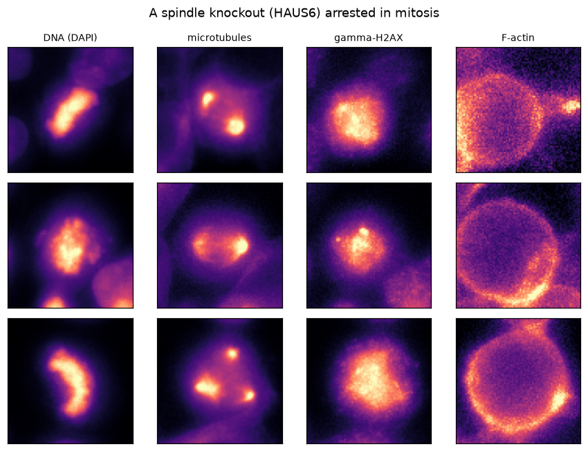
The arrest is visible in the cells themselves. A spindle-gene knockout (HAUS6) caught in mitosis shows the disorganized tubulin and condensed DNA of a cell that cannot divide, the pixels behind the G2M bar above.

show_cells(example_cells("HAUS6", n=3, phase="mitotic"), "A spindle knockout (HAUS6) arrested in mitosis")

The phenotypic landscape

The subset was a worked example of calling hits honestly. The reason to run a screen this size is the map it draws. With 5,049 genes measured in the same four channels (the published landscape’s 5,299 rows include 250 non-targeting guides), genes that do the same job look alike, and that similarity, computed from pixels alone, turns out to recover the cell’s known machinery. The published gene-level profiles carry the whole landscape, so the rest of this page works from them.

published = ad.read_h5ad(
    pooch.retrieve(
        "https://ops-explorer-public.s3.amazonaws.com/aconcagua/aconcagua/visualizations/interphase/aggregated_data.h5ad",
        known_hash="sha256:f55756939edc8ddf108092d88c4efe248765b4db4ec39322d4b4a988e04af929",
        fname="brief_interphase.h5ad",
    )
)
land = ad.AnnData(
    X=np.nan_to_num(np.asarray(published.X, dtype="float32")),
    obs=pd.DataFrame(
        {
            "Metadata_Gene": published.obs_names.astype(str),
            "cluster": published.obs["cluster_group_1"].astype(str).values,
        },
        index=published.obs_names.astype(str),
    ),
    var=published.var.copy(),
)
land.obsm["X_phate"] = np.asarray(published.obsm["X_phate"])
mt.tl.similarity(land, metric="pearson")  # gene x gene correlation in land.obsp["similarity"]
land

AnnData object with n_obs × n_vars = 5299 × 76
    obs: 'Metadata_Gene', 'cluster'
    var: 'feature_name', 'feature_type', 'compartment'
    uns: 'mantispy'
    obsm: 'X_phate'
    obsp: 'similarity'
    layers: None (.X)

Genes in the same complex look alike

Protein complexes are the sharpest test, because their subunits act as one machine, so knocking out any member gives the same phenotype. pathway_coherence() measures it: for each CORUM complex it compares the mean similarity among its members against random gene groups of the same size. The complexes come from corum(), in the source/target shape pathway_coherence reads. Ordering the most coherent complexes by membership turns the correlation matrix into blocks, and seen as distributions their subunits correlate several times more tightly than random gene pairs.

corum = mt.ds.corum()
present = set(land.obs_names)
comp = {
    c: [g for g in grp["target"].unique() if g in present]
    for c, grp in corum.groupby("source")
    if grp["target"].isin(present).sum() >= 4
}
in_corum = {g for ms in comp.values() for g in ms}

pos = {g: i for i, g in enumerate(land.obs_names)}
S = land.obsp["similarity"]
rng = np.random.default_rng(SEED)
random_pairs = S[rng.integers(0, S.shape[0], 20000), rng.integers(0, S.shape[0], 20000)]

mt.tl.pathway_coherence(
    land, corum, gene_key="Metadata_Gene", min_genes=4, n_permutations=1000, seed=SEED, metric="pearson"
)
pc = pd.DataFrame(land.uns["mantispy"]["pathway_coherence"])
print(f"CORUM complexes with 4+ members measured: {len(pc)}; coherent at q < 0.05: {int((pc['qvalue'] < 0.05).sum())}")

CORUM complexes with 4+ members measured: 430; coherent at q < 0.05: 179

top_sets = pc[(pc["n_genes"] >= 6) & (pc["n_genes"] <= 20)].sort_values("coherence", ascending=False)["set"].head(5)
members, bounds, labels = [], [0], []
for cx in top_sets:
    gs = [g for g in sorted(comp[cx]) if g not in members]
    if len(gs) < 4:
        continue
    members += gs
    bounds.append(len(members))
    labels.append(cx if len(cx) < 26 else cx[:24] + "...")
plot_complex_blocks(S, pos, members, bounds, labels, random_pairs)

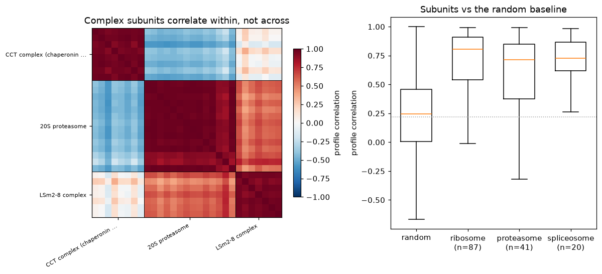
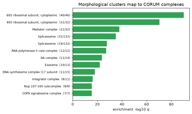
Well over a hundred of the measured complexes are coherent beyond chance. The published screen also groups the genes into clusters by morphology alone; testing each cluster against CORUM with an over-representation test (ora()) names them. Clusters built from pixels line up with real machinery, with no sequence or annotation used to build them.

mt.tl.ora(land, groupby="cluster", net=corum, gene_key="Metadata_Gene", tmin=4, padj_by="group")
ora = pd.DataFrame(land.uns["mantispy"]["ora"])
sizes = land.obs["cluster"].value_counts()
comp_size = {c: len(ms) for c, ms in comp.items()}
rows = []
for cl, grp in ora[ora["odds_ratio"] > 0].groupby("group"):
    if sizes.get(cl, 0) < 20:
        continue
    best = grp.sort_values("qvalue").iloc[0]
    if best["qvalue"] < 1e-3 and best["source"] in comp_size:
        rows.append(
            (
                cl,
                sizes[cl],
                best["source"],
                int(best["n"]),
                comp_size[best["source"]],
                -np.log10(max(float(best["qvalue"]), 1e-300)),
            )
        )
modules = pd.DataFrame(rows, columns=["cluster", "n", "complex", "k", "size", "neglog10q"]).sort_values("neglog10q")
plot_cluster_names(modules)

Placing genes into complexes

This is what the landscape is for. A cluster dominated by a complex also contains genes that are not CORUM members of it. If morphology tracks function, those genes are candidate partners of the machine their cluster names. Taking the best-named clusters and their non-member genes, mantispy places each candidate against the complex: its correlation to the known members sits at the members’ own level, far above random.

# Prefer complexes whose non-member candidates are not trivially named like the complex (e.g. rRNA processing,
# splicing and Golgi factors), which makes the prediction a real one rather than an obvious re-labelling.
WANT = ["rRNP", "Spliceosome", "COG", "exosome", "Integrator", "Mediator", "Nup", "proteasome"]
picks, used = [], set()
ranked = modules.sort_values("neglog10q", ascending=False)
for key in WANT:
    for _, r in ranked.iterrows():
        if key.lower() not in r["complex"].lower() or r["complex"] in used:
            continue
        members = list(land.obs_names[(land.obs["cluster"] == r["cluster"]).to_numpy()])
        cand = [g for g in members if g not in in_corum]
        known = [g for g in comp[r["complex"]] if g in pos]
        if len(cand) >= 3 and len(known) >= 4:
            picks.append((r["complex"], known, cand[:4]))
            used.add(r["complex"])
            break
    if len(picks) == 3:
        break

plot_candidates(picks, S, pos, random_pairs)
for cx, _known, cand in picks:
    print(f"{cx[:40]}: candidates {cand}")

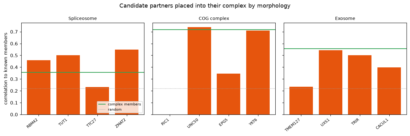
Spliceosome: candidates ['RBM42', 'TUT1', 'TTC27', 'ZMAT2']
COG complex: candidates ['RIC1', 'UNC50', 'EPG5', 'YKT6']
Exosome: candidates ['TMEM127', 'UXS1', 'TRIR', 'CACUL1']

The candidates are not noise. The spliceosome cluster pulls in splicing factors and the COG cluster pulls in Golgi-trafficking factors, genes a biologist would assign to the same machine. Most of these genes are already well characterised, and the clusters are named against CORUM, so this shows that morphology places genes with their machine. It does not show a function for a gene of unknown function; that use would need a candidate with no existing annotation.

Machines, not programs

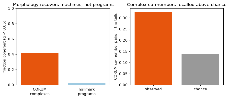
Not every gene set behaves this way. The broad transcriptional programs of the MSigDB hallmark collection, which group genes by co-expression rather than by a shared physical machine, are much less coherent in morphology. The screen sees what cells are built from, not what they transcribe. The same holds as a single retrieval number: known_relationships() counts how many CORUM co-member pairs land in the tails of the similarity distribution, and it beats a permutation null that shuffles the same annotation (the genome-wide number is modest because it mixes the tight machines with large, loose complexes that dilute it).

hallmark = mt.tl.gene_set_network("hallmark")
mt.tl.pathway_coherence(
    land,
    hallmark,
    gene_key="Metadata_Gene",
    min_genes=5,
    n_permutations=1000,
    seed=SEED,
    metric="pearson",
    key_added="pathway_coherence_hallmark",
)
ph = pd.DataFrame(land.uns["mantispy"]["pathway_coherence_hallmark"])

recall = mt.metrics.known_relationships(
    land, corum, label_key="Metadata_Gene", metric="pearson", n_permutations=200, seed=SEED
)
print(recall.to_string(index=False))
plot_machines(
    (pc["qvalue"] < 0.05).mean(), (ph["qvalue"] < 0.05).mean(), recall["value"].iloc[0], recall["null"].iloc[0]
)

             metric representation           key    value     null   pvalue
known_relationships              X Metadata_Gene 0.326356 0.136767 0.004975

What to take away

• In a pooled screen the guide is the unit and the well is the replicate.

• Targeting guides differ from non-targeting ones partly because of cutting alone. Unexpressed genes, which are cut but do nothing else, set the null for what lies beyond cutting, and it removes most of the random-gene calls.

• The features say which channels a knockout moved, and the single cells say which cell states it acted on.

• At screen scale, morphological similarity recovers protein complexes, the ribosome, proteasome and spliceosome among them, and places genes into the machines they resemble. That recovery is the evidence that the phenotypes mean something.