Where cells sit in the cycle

A knockout that stalls the cell cycle changes how much DNA its cells hold. This tutorial shows how to place single cells on the cycle with fit_cell_cycle() and project_cell_cycle(), and how to read what they write. How the cell-cycle model works explains each step of the model.

What you can learn depends on what you measured:

What you measured	What you get	How
a DNA stain	each cell’s phase probabilities, a position for S cells, the population prior for G1 and G2M cells, and the cells below 2N or above 4N	fit_cell_cycle(), project_cell_cycle()
other channels that change through the cycle	an experimental order of the cells within a phase	phase_order()
a marker of a phase, or a paired modality	a check of that order, and a split of G2M into G2 and mitosis	your own comparison

The cells come from an optical pooled CRISPR screen in HeLa cells (aconcagua_cells()). They are the cells of eight genes and the non-targeting controls, imaged in four channels: DAPI for DNA, gamma-H2AX for DNA damage, phalloidin for actin, and alpha-tubulin. Each gene’s function predicts a place in the cycle, so we state the predictions before looking:

Gene	Function	Prediction
RRM1	makes the nucleotides DNA replication needs	more cells in S
HAUS6, SKA2	build and attach the mitotic spindle	more cells in G2M
DTL	stops DNA from being copied twice in one cycle	more cells above 4N
PSMB7	a proteasome subunit, without which cells pile up before and in mitosis	more cells in G2M
SF3B3	a spliceosome subunit, whose loss stalls cells both in G1 and at G2 and M	more cells in G2M
ITGAV, TLN1	cell adhesion, with no known direct role in the cycle	the same as the controls

The optical pooled screens case study puts these genes in the context of the whole screen.

What the input needs

• The integrated intensity of a DNA stain, such as DAPI or Hoechst, per nucleus. It must be raw, since a normalized feature no longer doubles from G1 to G2. A pipeline that measured the image background should subtract it first.

• Reference cells that cycle in steady state, normally the negative controls.

• Groups within which the stain reads the same, to find the G1 peak in: the well in a pooled screen, where every well holds controls, or the plate in an arrayed screen.

• Optionally, the nuclear area and solidity, for the shape checks.

• Optionally, other channels for an order within a phase, and a marker to check it against.

import matplotlib.pyplot as plt
import numpy as np
import pandas as pd

import mantispy as mt

plt.rcParams["figure.dpi"] = 110

cells = mt.ds.aconcagua_cells()
print(cells.var["channel"].str.split("|").explode().value_counts().rename("features per channel").to_dict())
cells.obs["Metadata_Gene"].value_counts().rename("cells").to_frame().T

{'GH2AX': 355, 'DAPI': 353, 'PHALLOIDIN': 353, 'TUBULIN': 353}

Metadata_Gene	nontargeting	TLN1	SF3B3	HAUS6	ITGAV	PSMB7	RRM1	DTL	SKA2
cells	24166	2049	1984	1969	1921	1903	1890	1830	962

From the DNA stain alone

DNA content

dna_content() turns the integrated DAPI intensity into DNA content in doublings, the log2 of the intensity over that of the G1 peak. A G1 nucleus sits near 0, and a nucleus with twice that DNA sits near 1. We call the two amounts 2N and 4N, as is usual for the G1 and G2 DNA content, although HeLa cells are hypertriploid.

Staining differs between wells, so in a pooled screen the G1 peak is found per well, and reference="negcon" finds it on the non-targeting cells alone. A knockout that empties G1 then cannot move the peak of its well. In an arrayed screen, where a well holds one treatment, the controls of each plate set its peak instead:

mt.tl.dna_content(cells, dna_feature=..., by="Metadata_Plate", reference="negcon")

mt.tl.dna_content(
    cells,
    dna_feature="Nuclei_Intensity_IntegratedIntensity_DAPI",
    by=("Metadata_Plate", "Metadata_Well"),
    reference="negcon",
)

Fitting the cycle on the controls

fit_cell_cycle() checks that the controls cycle, then fits a G1 peak, S cells and a G2M peak to their DNA content, with a flat background for cells off the cycle. How the model works gives its assumptions. With qc_features, it also learns shape cutoffs from the controls, used further down.

mt.tl.fit_cell_cycle(cells, reference="negcon", qc_features=("Nuclei_AreaShape_Area", "Nuclei_AreaShape_Solidity"))
model = cells.uns["mantispy"]["cell_cycle"]
print("share of the cycle in G1, S and G2M:", np.round(np.diff(model["edges"]), 2))
pd.Series(
    {
        "passed the check": model["passed"],
        "2N peak (doublings)": round(model["peaks"][0], 3),
        "4N peak (doublings)": round(model["peaks"][1], 3),
        "2N peak width (doublings)": round(model["sd"], 3),
        "share of cells in G1": round(model["fractions"][0], 2),
        "share of cells in S": round(model["fractions"][1], 2),
        "share of cells in G2M": round(model["fractions"][2], 2),
        "share of cells off the cycle": round(model["off_cycle"], 3),
    }
)

share of the cycle in G1, S and G2M: [0.57 0.3  0.14]

passed the check                 True
2N peak (doublings)            -0.005
4N peak (doublings)              0.92
2N peak width (doublings)       0.096
share of cells in G1             0.65
share of cells in S              0.25
share of cells in G2M             0.1
share of cells off the cycle    0.023
dtype: object

The controls pass the check. Their 2N peak sits at -0.005 doublings and their 4N peak at 0.92, short of 1. One cause is an image background that was not subtracted, as how the model works shows. Of the control cells on the cycle, 65% are in G1, 25% in S and 10% in G2M, and 2.3% of all control cells sit off the cycle. Converted with the age distribution of a growing population, the three shares become 57%, 30% and 14% of the cycle, kept in model["edges"]. A position is a fraction of the cycle, not a time in hours.

project_cell_cycle() places every cell, knockouts included, on the controls’ model. It writes:

• obsm["cell_cycle_probabilities"]: the probability of G1, S, G2M, sub-2N and above-4N;

• obs["cell_cycle_phase"]: the most probable of the five, a convenience for counting;

• obs["cell_cycle_position"] and obsm["cell_cycle_quantiles"]: the median of the posterior position and its 5%, 25%, 75% and 95% quantiles, for cells on the cycle;

• obs["cell_cycle_qc"]: the shape checks, further down;

• uns["mantispy"]["cell_cycle_wells"]: a check of each well’s stain, further down.

mt.tl.project_cell_cycle(cells)
example = cells.obs.groupby("cell_cycle_phase", observed=True).head(1).index
pd.concat(
    [
        cells.obs.loc[example, ["Metadata_DNAContent", "cell_cycle_phase"]],
        cells.obsm["cell_cycle_probabilities"].loc[example],
        cells.obsm["cell_cycle_quantiles"].loc[example],
    ],
    axis=1,
).round(2)

	Metadata_DNAContent	cell_cycle_phase	G1	S	G2M	sub-2N	above-4N	5%	25%	50%	75%	95%
0	0.14	G1	0.79	0.20	0.00	0.00	0.00	0.03	0.16	0.33	0.53	0.62
1	0.27	S	0.13	0.85	0.00	0.02	0.00	0.18	0.61	0.63	0.65	0.68
3	1.00	G2M	0.00	0.18	0.81	0.00	0.01	0.83	0.87	0.91	0.96	0.99
5	1.45	above-4N	0.00	0.00	0.00	0.00	1.00	NaN	NaN	NaN	NaN	NaN
205	-0.84	sub-2N	0.00	0.00	0.00	1.00	0.00	NaN	NaN	NaN	NaN	NaN

The stain check could not judge two of the wells. The checks further down come back to them.

In the table, a cell at 0.14 doublings is in G1 with probability 0.79 and in S with 0.20, since a cell early in S holds little more DNA than one in G1. A cell at 0.27 doublings is in S with probability 0.85, and the middle half of its posterior spans 0.61 to 0.65 of the cycle. A cell at 1.00 doublings is in G2M with probability 0.81, and the middle half of its posterior spans 0.87 to 0.96, most of G2M. The cells at 1.45 and -0.84 doublings sit above 4N and below 2N, and have no position.

So the position means something per cell only in S. Within G1 and G2M it is the population prior, as the posterior for one cell shows. Don’t correlate it with morphology inside those phases.

controls = cells[cells.obs["Metadata_Control_Type"] == "negcon"]
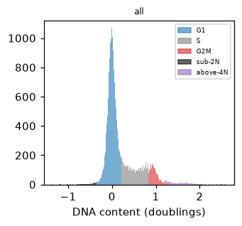
mt.pl.cell_cycle(controls, dna_feature="Metadata_DNAContent", by=None)
plt.gca().set_xlabel("DNA content (doublings)")
plt.show()
controls.obs["cell_cycle_phase"].value_counts(normalize=True).round(3)

cell_cycle_phase
G1          0.670
S           0.196
G2M         0.120
above-4N    0.011
sub-2N      0.004
Name: proportion, dtype: float64

Counted by their most probable phase, 67% of control cells are in G1, 20% in S, 12% in G2M, 1.1% above 4N and 0.4% below 2N. The counted shares differ a little from the fitted ones, since the most probable phase gives some early S cells to G1 and some late S cells to G2M.

The cell-cycle clock

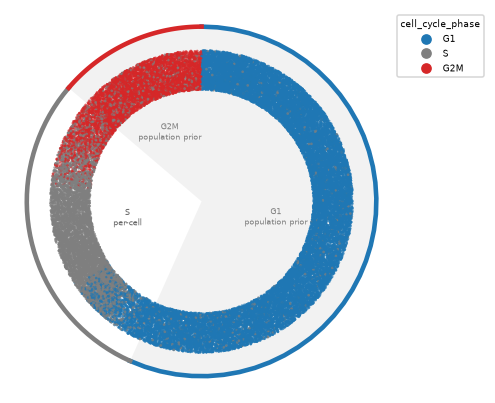
cell_cycle_clock() draws the placement as a ring, with position 0 at the top. Each cell’s angle is a position drawn from its posterior, so the ring fills. The S arc places each cell from its own DNA, and the G1 and G2M arcs are shaded and labeled as the population prior.

mt.pl.cell_cycle_clock(cells)

The same placement reads as a density with kind="rings". The drawn positions are smoothed into one curve over every cell, filled by phase, and the dashed circle marks the height the curve would have if the cells spread evenly over the cycle. The smoothing wraps across division, so the end of G2M runs into the start of G1.

mt.pl.cell_cycle_clock(cells, kind="rings")

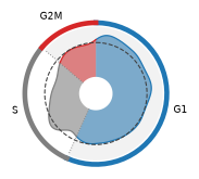
The curve rises above the dashed circle early in G1 and falls back to it late in G1, because the population prior puts a cell early in G1 more often than late. Within the G1 and G2M arcs the shape comes from the prior, not from the cells, so read how much of the curve sits in each arc rather than its shape there. The S arc places each cell from its own DNA.

Shape checks

With qc_features, obs["cell_cycle_qc"] gives the first shape check a nucleus fails, with cutoffs learned from the controls (why):

• "irregular": a solidity, the nucleus’ area over that of its convex hull, below the controls’;

• "small": an area below the controls’;

• "dim": too little DNA per area;

• "ok": none of these.

Mitotic cells condense their chromosomes, so they can fail the same checks as merged nuclei and fragments. Whether to drop flagged cells depends on the cell line and the question, and checks= in project_cell_cycle() picks the checks to apply. The screen’s image classifier, whose interphase and mitotic calls are in Metadata_Class, shows what the flags catch in these HeLa cells.

mitotic = cells.obs["Metadata_Class"] == "Mitotic"
pd.crosstab(cells.obs["cell_cycle_qc"], np.where(mitotic, "mitotic", "interphase"), normalize="columns").round(3)

col_0	interphase	mitotic
cell_cycle_qc
ok	0.982	0.458
irregular	0.016	0.410
small	0.001	0.132
dim	0.000	0.000

The checks pass 98% of interphase cells but flag 54% of the cells the classifier calls mitotic, 41% as irregular and 13% as small. Dropping flagged cells here would remove about half of the mitoses, so the rest of the tutorial keeps every cell.

Effects of the knockouts

The DNA content of each gene’s cells, colored by phase, shows the effects before any test.

mt.pl.cell_cycle(cells, dna_feature="Metadata_DNAContent", by="Metadata_Gene", ncols=3)
for axis in plt.gcf().axes:
    axis.set_xlabel("DNA content (doublings)")
plt.show()

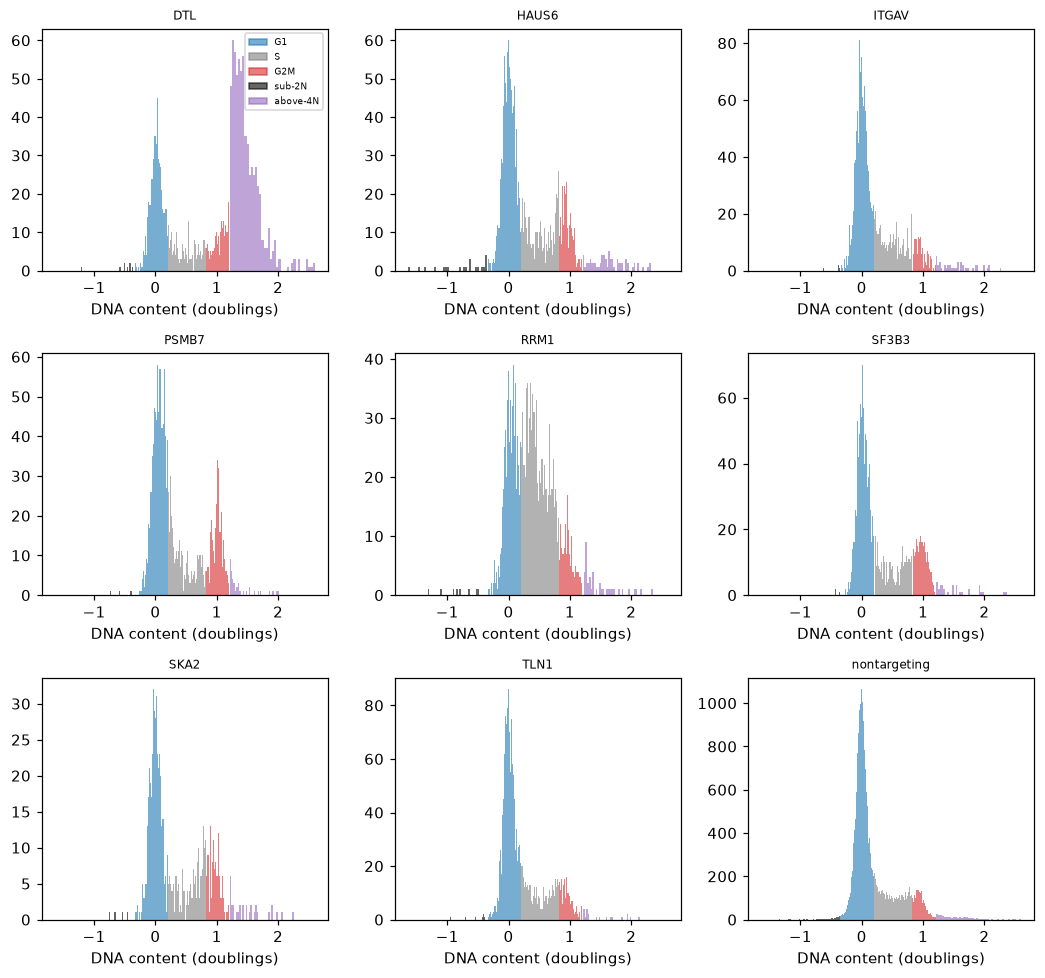
RRM1 has more cells in S, DTL more above 4N, and PSMB7 and SF3B3 a higher 4N peak. HAUS6 adds some cells above 4N as well as at 4N, while ITGAV and TLN1 look like the controls.

composition_shift() tests each gene’s phase shares against the controls’. It compares shares within each well of each plate and takes the guide as the unit. The p-value comes from relabeling whole guides, since cells of one guide share the guide’s efficiency and are not independent. With 999 permutations, a p-value cannot go below 0.001, and four guides per gene limit how small an effect the test can find.

In the first table, the gain is the change in the share of cells whose most probable phase is the predicted one, and the expected gain counts each cell by its probabilities instead. The distance is the total variation distance over all five phases. A prediction holds when the q-value is below 0.05 and the predicted phase gains more than 5 percentage points. For ITGAV and TLN1 it holds when the q-value is 0.05 or more. The second table gives the change in every phase.

mt.tl.composition_shift(
    cells, key="cell_cycle_phase", groupby="Metadata_Gene", replicate="Metadata_sgRNA", n_permutations=999
)
shift = cells.uns["mantispy"]["composition_shift"].set_index("group")
gene = cells.obs["Metadata_Gene"].astype(str).to_numpy()
soft = cells.obsm["cell_cycle_probabilities"].groupby(gene).mean()
soft_change = soft - soft.loc["nontargeting"]

predicted = {
    "RRM1": "S",
    "HAUS6": "G2M",
    "SKA2": "G2M",
    "DTL": "above-4N",
    "PSMB7": "G2M",
    "SF3B3": "G2M",
    "ITGAV": None,
    "TLN1": None,
}
rows = []
for name, phase in predicted.items():
    significant = shift.loc[name, "qvalue"] < 0.05
    rows.append(
        {
            "gene": name,
            "predicted phase": phase or "no change",
            "gain in that phase": shift.loc[name, phase] if phase else np.nan,
            "expected gain": soft_change.loc[name, phase] if phase else np.nan,
            "distance": shift.loc[name, "distance"],
            "qvalue": shift.loc[name, "qvalue"],
            "holds": bool(significant and shift.loc[name, phase] > 0.05) if phase else not significant,
        }
    )
pd.DataFrame(rows).set_index("gene").round(3)

	predicted phase	gain in that phase	expected gain	distance	qvalue	holds
gene
RRM1	S	0.278	0.255	0.322	0.003	True
HAUS6	G2M	0.097	0.078	0.135	0.024	True
SKA2	G2M	0.108	0.090	0.152	0.003	True
DTL	above-4N	0.352	0.347	0.414	0.003	True
PSMB7	G2M	0.136	0.108	0.146	0.010	True
SF3B3	G2M	0.115	0.092	0.120	0.036	True
ITGAV	no change	NaN	NaN	0.033	0.420	True
TLN1	no change	NaN	NaN	0.034	0.420	True

shift[["G1", "S", "G2M", "sub-2N", "above-4N"]].round(3)

	G1	S	G2M	sub-2N	above-4N
group
PSMB7	-0.137	-0.008	0.136	-0.001	0.010
DTL	-0.332	-0.082	0.061	0.001	0.352
SF3B3	-0.110	-0.009	0.115	-0.001	0.005
SKA2	-0.152	0.018	0.108	0.000	0.025
HAUS6	-0.135	0.009	0.097	0.006	0.024
ITGAV	-0.027	0.021	-0.006	-0.000	0.012
TLN1	-0.033	0.007	0.027	-0.000	-0.001
RRM1	-0.322	0.278	0.032	0.001	0.010

Every predicted gain is significant, and ITGAV and TLN1 show no significant change. RRM1 gains 28 percentage points of its cells in S, and DTL gains 35 above 4N. HAUS6, SKA2, PSMB7 and SF3B3 gain 10 to 14 points in G2M, with q-values from 0.003 to 0.036. ITGAV and TLN1 sit at a total variation distance of 0.03 from the controls, with q-values of 0.42. No change was found, which does not show that there is none.

SF3B3’s G1 share falls by 11 points rather than rising, so of the stall in G1 and at G2 and M that its function predicts, only the G2 and M part shows. The PSMB7 cells imaged are those that survived losing the proteasome, so its shares may understate the arrest.

The guides of a gene should agree. The table gives each guide’s share of cells per phase.

per_guide = pd.crosstab(
    [cells.obs["Metadata_Gene"], cells.obs["Metadata_sgRNA"]], cells.obs["cell_cycle_phase"], normalize="index"
)
per_guide.drop(index="nontargeting", level=0).round(2)

	cell_cycle_phase	G1	S	G2M	sub-2N	above-4N
Metadata_Gene	Metadata_sgRNA
DTL	ACAGCTGTATT	0.27	0.09	0.22	0.00	0.42
	AGGTGATAAAC	0.47	0.14	0.17	0.01	0.21
	TGAAGCTGCCT	0.31	0.11	0.16	0.01	0.41
	TTTCCAGCAAA	0.30	0.14	0.14	0.00	0.42
HAUS6	AAATTATATGA	0.33	0.22	0.36	0.03	0.06
	AACTTGAGATC	0.62	0.20	0.15	0.00	0.02
	ATGCATTTGTG	0.58	0.20	0.18	0.01	0.03
	CTGATTCCTTA	0.51	0.22	0.22	0.01	0.03
ITGAV	AACGATGAGCT	0.69	0.20	0.10	0.00	0.01
	AAGTTACTTCG	0.65	0.21	0.11	0.01	0.03
	AGAACATGACT	0.63	0.21	0.12	0.00	0.04
	GCACCTCTCTT	0.62	0.24	0.12	0.00	0.02
PSMB7	AACTGGCACGA	0.40	0.23	0.33	0.00	0.04
	GAAAACGTTAC	0.48	0.21	0.28	0.00	0.03
	GCAGATACAAG	0.62	0.15	0.21	0.01	0.01
	TAAGTTGCCTT	0.54	0.19	0.25	0.00	0.02
RRM1	CCTACCTAGAA	0.29	0.48	0.20	0.00	0.02
	CTTGTACCCCA	0.32	0.52	0.13	0.00	0.03
	GTAATCCAAGG	0.31	0.55	0.11	0.01	0.02
	TGGCAAACACT	0.43	0.38	0.16	0.01	0.02
SF3B3	AAGAATAGCTC	0.43	0.18	0.38	0.00	0.02
	AGCAGACAATG	0.66	0.17	0.16	0.01	0.01
	CCACAGGCCAC	0.44	0.23	0.31	0.00	0.02
	TGAGCCGGATC	0.52	0.18	0.28	0.00	0.01
SKA2	CAACAGCAACT	0.47	0.26	0.23	0.00	0.03
	GGATTACATTC	0.52	0.21	0.25	0.01	0.01
	GGTCGATAAGC	0.50	0.17	0.32	0.01	0.00
	TCATCCTGATT	0.58	0.17	0.20	0.00	0.04
TLN1	AACTGTGAAGA	0.60	0.23	0.16	0.00	0.02
	CAAGCTTAAAC	0.66	0.18	0.15	0.00	0.01
	GCGGCAGGCGT	0.70	0.19	0.10	0.01	0.01
	GGAAGAACAAG	0.64	0.18	0.17	0.00	0.01

The guides mostly agree, but several genes have one guide that differs. One HAUS6 guide, AAATTATATGA, has 36% of its cells in G2M against 15% to 22% for the other three, and one SF3B3 guide, AGCAGACAATG, looks close to the controls. One DTL guide has 21% of its cells above 4N against 41% to 42% for the others, and one RRM1 guide 38% in S against about half.

Checks on the measurement

The well check locates each well’s 2N and 4N peaks. If both sit off the controls’ peaks by the same amount, the well reads its DNA stain differently, and every position in it carries that shift. A warning names any well shifted by more than the width of the 2N peak. A well with only one of the two peaks, such as one where a knockout arrested every cell, cannot tell a shifted stain from a shifted population, so it is not judged and its shift is missing. The positions are never corrected.

wells = cells.uns["mantispy"]["cell_cycle_wells"]
print(f"{wells['shift'].notna().sum()} of {len(wells)} wells checked; the 2N peak width is {model['sd']:.3f} doublings")
print("not judged:", wells.loc[wells["shift"].isna(), ["Metadata_Plate", "Metadata_Well"]].to_numpy().tolist())
judged = wells.dropna(subset=["shift"]).sort_values("shift")
judged.round(3).iloc[[0, 1, -2, -1]]

44 of 46 wells checked; the 2N peak width is 0.096 doublings
not judged: [['6', 'B01'], ['7', 'A02']]

	Metadata_Plate	Metadata_Well	n_cells	shift
41	8	A02	858	-0.080
40	8	A01	857	-0.062
37	7	B01	860	0.040
10	2	B02	850	0.065

The check judged 44 of the 46 wells. Well B01 on plate 6 shows no 4N peak the check can find, and in well A02 on plate 7 the gap between the peaks differs from the controls’. The largest shift, -0.080 doublings, is smaller than the 2N peak width, so no well was flagged. Only small shifts are expected here, since each well’s G1 peak was set by its own non-targeting cells. In an arrayed screen, with by="Metadata_Plate", a well that stains differently from the rest of its plate would show up in this check.

When the check fails

The cycle model needs a reference that cycles. A reference that does not, such as the RRM1 knockouts with their cells spread through S, fails the check, and the model is marked as failed.

cells.obs["is_RRM1"] = (cells.obs["Metadata_Gene"] == "RRM1").to_numpy()
mt.tl.fit_cell_cycle(cells, reference="is_RRM1", key_added="rrm1_model")
pd.Series(cells.uns["mantispy"]["rrm1_model"]["check"])

WARNING  fit_cell_cycle: the reference shows no separate 2N and 4N peaks, so project_cell_cycle will give NaN      

is_peak            False
peak_ratio      0.638471
valley_ratio    1.154976
s_floor         0.902673
s_share         0.363492
dtype: object

The warning says the reference shows no separate 2N and 4N peaks. The model keeps the measures of the check in check, and projecting with a failed model gives NaN for every cell. RRM1’s S cells fill the gap between the peaks, so the valley is higher than the 4N peak, a ratio of 1.155, and the 4N density is no peak of its own. The Notes of fit_cell_cycle() list the criteria, and how the model works shows passing and failing populations. When the controls themselves fail, check that the input is the raw integrated intensity, that by matches the screen, and that the controls are cycling cells. If the stain does not resolve a 4N peak at all, dna_state() still calls cells 2N, S or 4N from fixed gates on the DNA content, without positions.

With other channels: an order within a phase

DNA content cannot order cells within G1 or G2M, but the other channels may. phase_order() orders the cells of one phase without labels. It fits an axis of progress through S from the other features on the controls, carries it into the phase, smooths it along the cells’ nearest neighbors, and places every cell of the phase against the controls. How the cell-cycle model works shows each step, and where it worked and where it did not.

The order is experimental, and every call warns. The table sums each channel’s feature weights.

mt.tl.phase_order(cells, phase="G2M")
entry = cells.uns["mantispy"]["cell_cycle_G2M_order"]
weights = pd.Series(entry["weights"], index=entry["features"])
channel = cells.var.loc[weights.index, "channel"]
pd.DataFrame(
    {
        "summed weight": weights.groupby(channel).sum(),
        "largest weight": weights.groupby(channel).max(),
        "features": weights.groupby(channel).size(),
    }
).sort_values("summed weight", ascending=False).round(2)

	summed weight	largest weight	features
channel
GH2AX	75.49	0.58	289
TUBULIN	27.96	0.19	286
PHALLOIDIN	16.21	0.14	287
GH2AX|PHALLOIDIN	2.82	0.45	18
TUBULIN|GH2AX	2.75	0.45	18
TUBULIN|PHALLOIDIN	0.97	0.15	18

Gamma-H2AX carries most of the weight, then tubulin and phalloidin. Each weight is a feature’s rank correlation with DNA content in S, and gamma-H2AX features reach 0.58, so the order within G2M here is largely an order of gamma-H2AX, a marker of DNA damage. The five features with the largest weights all measure it.

weights.sort_values(ascending=False).head(5).round(3)

Cells_Texture_SumVariance_GH2AX_5                0.578
Cells_Texture_Variance_GH2AX_5                   0.575
Cells_Intensity_StdIntensity_GH2AX               0.575
Nuclei_Intensity_UpperQuartileIntensity_GH2AX    0.536
Cells_PFTAS_Stat45_GH2AX                         0.535
dtype: float64

A knockout that damages DNA will then read as late in G2M, whether or not its cells are.

With a marker: checking the order

The screen’s image classifier labels each cell interphase or mitotic, in Metadata_Class. An order that follows progress puts mitotic cells late. The labels serve here only as that check.

from sklearn.metrics import roc_auc_score

in_g2m = (cells.obs["cell_cycle_phase"] == "G2M").to_numpy()
check = in_g2m & (cells.obs["Metadata_Control_Type"] == "negcon").to_numpy()
order = cells.obs["cell_cycle_G2M_order"].to_numpy()
print(
    f"AUROC of the G2M order for mitotic calls, control cells in G2M: {roc_auc_score(mitotic[check], order[check]):.2f}"
)
quarter = pd.qcut(order[check], 4, labels=["first", "second", "third", "fourth"])
pd.Series(mitotic[check].to_numpy()).groupby(quarter, observed=True).mean().rename("share mitotic").round(3)

AUROC of the G2M order for mitotic calls, control cells in G2M: 0.88

first     0.050
second    0.058
third     0.338
fourth    0.762
Name: share mitotic, dtype: float64

On the controls the order does follow mitosis. Mitotic cells sit late, with an AUROC of 0.88, and the share of mitotic cells rises from 5% in the first quarter of the order to 76% in the last. The check covers one dataset, the only one here with a label.

With the order present, the clock places G2M cells along their arc by it and labels the arc as the experimental order. Highlighting the classifier’s mitotic calls among the controls shows where they land.

controls = cells[cells.obs["Metadata_Control_Type"] == "negcon"]
mt.pl.cell_cycle_clock(controls, color="Metadata_Class", groups=["Mitotic"])

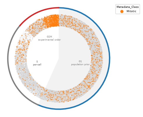
Mitotic calls pile up at the late end of the G2M arc, just before division. Others spread over the G1 arc, where the angle follows the prior, and some fall in S.

Across the knockouts, the order and the mitotic share disagree. The table gives, for each gene’s G2M cells, the median order, the share the classifier calls mitotic, and the median nuclear gamma-H2AX.

gh2ax = cells[:, "Nuclei_Intensity_MeanIntensity_GH2AX"].to_df().iloc[:, 0]
g2m_cells = cells.obs.loc[in_g2m]
pd.DataFrame(
    {
        "median order in G2M": g2m_cells.groupby("Metadata_Gene", observed=True)["cell_cycle_G2M_order"].median(),
        "share mitotic in G2M": mitotic[in_g2m].groupby(g2m_cells["Metadata_Gene"], observed=True).mean(),
        "median nuclear gamma-H2AX in G2M": gh2ax[in_g2m].groupby(g2m_cells["Metadata_Gene"], observed=True).median(),
    }
).sort_values("median order in G2M").round(3)

	median order in G2M	share mitotic in G2M	median nuclear gamma-H2AX in G2M
Metadata_Gene
PSMB7	0.251	0.068	1414.047974
DTL	0.481	0.055	1730.063965
nontargeting	0.487	0.302	1722.130981
ITGAV	0.560	0.226	1810.863037
TLN1	0.586	0.332	1857.599976
HAUS6	0.619	0.637	1924.536987
SKA2	0.635	0.560	1932.307007
RRM1	0.713	0.087	2519.260986
SF3B3	0.860	0.277	2985.529053

SF3B3’s G2M cells sit latest in the order, at a median of 0.86, yet 28% of them are mitotic, about as many as the controls’ 30% at 0.49. They carry the most gamma-H2AX. RRM1’s G2M cells sit at 0.71 with 9% mitotic, and also carry more gamma-H2AX than the controls. PSMB7’s sit earliest, at 0.25, with the least gamma-H2AX. HAUS6 and SKA2, whose G2M cells are 64% and 56% mitotic, sit at 0.62 and 0.64, later than the controls. Sorted by median order, the genes are also sorted by gamma-H2AX, except that DTL and the controls swap, and the mitotic share follows no such order. Read it as progress only for knockouts that leave DNA damage alone, and check any reading against the mitotic share.

Highlighting three of the knockouts on the clock, against a gray background of all the other cells, shows where each one lands.

mt.pl.cell_cycle_clock(cells, color="Metadata_Gene", groups=["RRM1", "HAUS6", "DTL"])

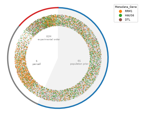
Many of RRM1’s cells sit on the S arc, and its G2M cells sit late in the order. HAUS6’s G2M cells sit late as well, as cells held in mitosis should. DTL’s cells on the cycle lean toward G2M, and its largest effect, the cells above 4N, is off the ring, since those cells have no position.

The classifier also splits each gene’s G2M calls into G2 and mitosis (M), which suggests which knockouts hold cells in mitosis and which before it. The split covers only cells called G2M. A quarter of the cells the classifier calls mitotic are called G1 (second table), so the gains in M likely understate the change.

called = cells.obs["cell_cycle_phase"].astype(str)
split = called.where(called != "G2M", np.where(mitotic, "M", "G2"))
by_gene = pd.crosstab(cells.obs["Metadata_Gene"], split, normalize="index")[
    ["G1", "S", "G2", "M", "sub-2N", "above-4N"]
]
(by_gene - by_gene.loc["nontargeting"]).round(3)

cell_cycle_phase	G1	S	G2	M	sub-2N	above-4N
Metadata_Gene
DTL	-0.330	-0.082	0.087	-0.026	0.001	0.350
HAUS6	-0.137	0.011	-0.006	0.101	0.007	0.024
ITGAV	-0.027	0.020	0.006	-0.010	-0.000	0.012
PSMB7	-0.138	-0.009	0.155	-0.019	-0.001	0.011
RRM1	-0.321	0.278	0.055	-0.023	0.001	0.010
SF3B3	-0.112	-0.010	0.088	0.029	-0.001	0.005
SKA2	-0.133	0.005	0.015	0.090	0.001	0.021
TLN1	-0.033	0.007	0.015	0.013	-0.000	-0.001
nontargeting	0.000	0.000	0.000	0.000	0.000	0.000

pd.crosstab(cells.obs["cell_cycle_phase"], cells.obs["Metadata_Class"], normalize="columns").round(3)

Metadata_Class	Interphase	Mitotic
cell_cycle_phase
G1	0.645	0.248
S	0.213	0.137
G2M	0.113	0.505
sub-2N	0.003	0.016
above-4N	0.025	0.093

HAUS6 and SKA2 gain 10 and 9 percentage points of their cells in mitosis and almost none in G2, consistent with an arrest in mitosis, as spindle defects predict. Both also gain about 2 points above 4N, as cells that leave a mitotic arrest without dividing would. PSMB7 gains 16 points in G2 and has slightly fewer cells in mitosis than the controls, and DTL gains 9 points in G2, consistent with an arrest before mitosis. For PSMB7 that matches only the G2 half of the prediction. SF3B3 gains 9 points in G2 and 3 in mitosis. Half of the cells the classifier calls mitotic (51%) are in G2M, and a quarter (25%) sit at 2N, possibly anaphase figures segmented as two nuclei, or classifier errors.

Comparing knockouts as densities

Markers of several knockouts stack on top of each other on one clock. With kind="rings", each gene’s cells on the cycle become one smoothed density on its own ring, in the order of groups, the first outermost. reference="nontargeting" adds the controls as the first ring, in gray, and draws their density as the dashed line of every ring, so a knockout’s excess in a phase shows where its ring rises above the dashed line. Because each density sums to one, a rise in one arc comes with a dip elsewhere. Each density covers only the gene’s cells on the cycle, so it shows how they spread over the cycle, while the tables above give the shares including the cells off it.

mt.pl.cell_cycle_clock(
    cells, kind="rings", color="Metadata_Gene", groups=["RRM1", "HAUS6", "DTL"], reference="nontargeting"
)

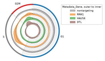
RRM1’s ring rises above the controls through S, which is the gain in S the composition test found. HAUS6’s rises late in G2M, and DTL’s rises in G2M as well. DTL’s cells above 4N, its largest effect, are off the cycle and so not in its ring. Since phase_order() has run, the G2M arc follows the experimental order instead of the prior, so where a density sits within G2M comes from that order, which here mostly tracks gamma-H2AX (see above).

To see every gene at once, groupby= draws one small clock per gene, each filled by phase, with the controls’ density as the dashed line and the controls’ own clock first.

mt.pl.cell_cycle_clock(cells, kind="rings", groupby="Metadata_Gene", reference="nontargeting")

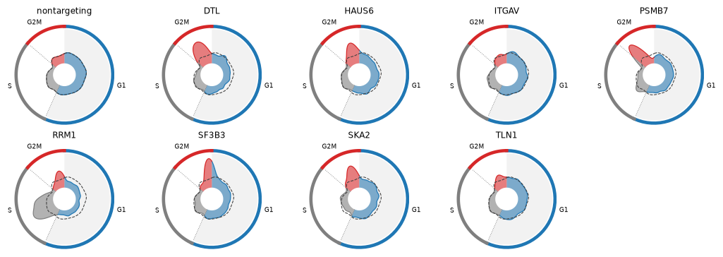
The small clocks sort the knockouts by eye. RRM1 is the only gene with a large bulge in S. PSMB7’s G2M density sits at the start of the arc, and SF3B3’s and SKA2’s toward its end, as their median G2M orders of 0.25, 0.86 and 0.64 in the table above say. ITGAV and TLN1 stay close to the dashed line, where their composition test found no significant change. All clocks share one scale, so the area of a bulge compares across genes as a share of each gene’s cells on the cycle. DTL’s G2M bulge leaves out its many cells above 4N, and the tables above give the shares of all cells.

Rings get thin with many knockouts. kind="ridge" draws the same densities as rows over a straight cycle axis, one row per gene, which stays readable for a whole screen.

mt.pl.cell_cycle_clock(cells, kind="ridge", color="Metadata_Gene", reference="nontargeting")

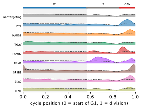
The rows make the order within G2M easier to compare. PSMB7 peaks early in the G2M arc, DTL in its middle, and HAUS6, SKA2 and SF3B3 late. For HAUS6 and SKA2, most of whose G2M cells are mitotic, late means close to division. SF3B3’s G2M cells are no more often mitotic than the controls’ and carry the most gamma-H2AX, so its late peak reflects DNA damage rather than progress. RRM1 peaks in the first half of S and again late in G2M, where it also carries more gamma-H2AX than the controls. Because the smoothing wraps across division, SF3B3’s pile-up at the end of G2M also shows at the start of G1. Within G1 the positions follow the prior, so the rows differ there mostly in height.

DTL’s nuclei above 4N

Merged nuclei and mitotic figures can also sit above 4N, and shape and the classifier together tell them from single nuclei with extra DNA. Cells that died before imaging are missing altogether, so a knockout that kills its arrested cells shows fewer of them than it made.

shape = cells[:, ["Nuclei_AreaShape_Area", "Nuclei_AreaShape_Solidity"]].to_df()
above = (cells.obs["cell_cycle_phase"] == "above-4N").to_numpy()
pd.DataFrame(
    {
        "nuclei above 4N": pd.Series(above).groupby(gene).sum(),
        "median area": shape.loc[above, "Nuclei_AreaShape_Area"].groupby(gene[above]).median(),
        "median solidity": shape.loc[above, "Nuclei_AreaShape_Solidity"].groupby(gene[above]).median(),
        "share irregular": (cells.obs.loc[above, "cell_cycle_qc"] == "irregular").groupby(gene[above]).mean(),
        "share mitotic": mitotic[above].groupby(gene[above]).mean(),
    }
).round(3)

	nuclei above 4N	median area	median solidity	share irregular	share mitotic
DTL	660	2660.5	0.980	0.014	0.005
HAUS6	69	2058.0	0.960	0.435	0.884
ITGAV	43	2163.0	0.963	0.442	0.302
PSMB7	42	2467.0	0.979	0.095	0.119
RRM1	40	2625.5	0.975	0.300	0.325
SF3B3	32	1916.5	0.967	0.375	0.531
SKA2	31	1913.0	0.965	0.323	0.677
TLN1	21	1939.0	0.966	0.333	0.429
nontargeting	261	1959.0	0.959	0.479	0.598

DTL’s 660 nuclei above 4N look like single, large nuclei. Their median solidity is 0.980 and their median area 2,660 pixels, against 0.959 and 1,959 pixels for the controls’ 261, and fewer than 1% of them are mitotic. The controls’ nuclei above 4N are mostly mitotic figures or merged nuclei, since 60% of them are mitotic and 48% are irregular. So DTL’s excess above 4N comes from single nuclei, as re-replication would produce, not from merged nuclei.